10 tricks of MS Excel that you must know

Introduction

Microsoft Excel is an integral part of most businesses. Some people relish the capabilities of Excel, finding it a useful tool that allows them to easily manage, report on and illustrate tables of data.

Others, however, find it tedious and downright obtuse, unable to make heads or tails of what exactly Excel can do from them, aside from keeping things in neat columns and rows.

Below is a list of 10 easy tricks, shortcuts and hacks that will put you on the path to being an Excel super user.

(Note: There are a many versions of Excel, including versions for desktop (Windows, Mac OS X) and mobile (iOS and Android) operating systems. The visuals are screenshots from a Mac version of Excel. These tips were confirmed to work on a Mac and Windows desktop, but may apply to other versions as well. This piece also discusses keyboard shortcuts for use in a Windows OS. For Mac, replace the “Control” key with the “Command” key.)

MS Excel Tips and Tricks

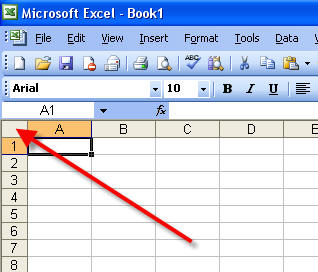
Select All Cells in a Spreadsheet at Once

Do you need to reformat your font or make some other sweeping change to your Excel workbook? An easy way to select all the cells in the document is to click on the square in the upper left-hand corner where the top of the rows and columns meet.

Copy a Worksheet From 1 Workbook to Another

This is helpful if you’re looking to merge data across two workbooks together and don’t want to reformat all of your data in either workbook.

1. 1. 1. 1. Start by opening your “source” workbook (the one with the data you want to copy).
         2. Next, open your “target” workbook (you want to copy to). This can be a new workbook or an existing workbook.
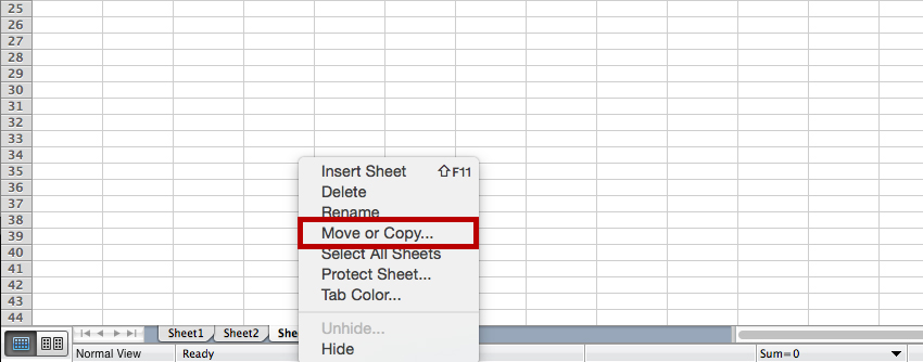
         3. In your source workbook, look towards the bottom left-hand corner and find the name of the sheet you want to copy. Unless the name of the worksheet is changed, it should have a name like “Sheet1” or something else.
         4. Right-click on the sheet you want to copy (if on a Mac with a single-button mouse, you may need to hold down the Control key while clicking).
         5. Select “Move or Copy …” from the menu.

      

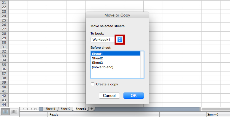
      6. From the list, select where you want to move or copy the sheet to. You’ll need to click on the dropdown                            at the top to see other open workbooks.

   2.                       7. Choose the workbook to copy it to and where in the order of the existing worksheets you want it to be.

Alternatively, you can simply move the worksheet from one workbook to another by dragging it with your mouse, but it might be safer to copy it, at least until your comfort level with Excel increases.

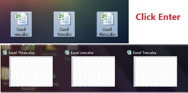
Open Excel Files in Bulk

Rather than open files one by one when you have multiple files you need to handle, there is a handy way to open them all with one click. Select the files you would like to open then press the Enter key on the keyboard, all files will open simultaneously

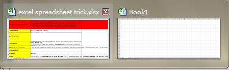
Shift Between Different Excel Files

When you have different spreadsheets open, it’s really annoying shifting between different files because sometimes working on the wrong sheet can ruin the whole project. Using Ctrl + Tab you can shift between different files freely. This function is also applicable to other files like different Windows tabs in Firefox when opened using Windows 7.

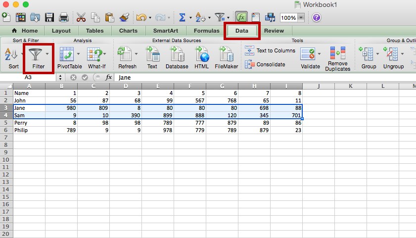
Filtering Data

By clicking on the “Data” tab at the top of the page and then clicking “Filter,” you will give each column it’s own clickable dropdown menu on each cell in the first row. Click one, and you can sort data in a variety of ways.

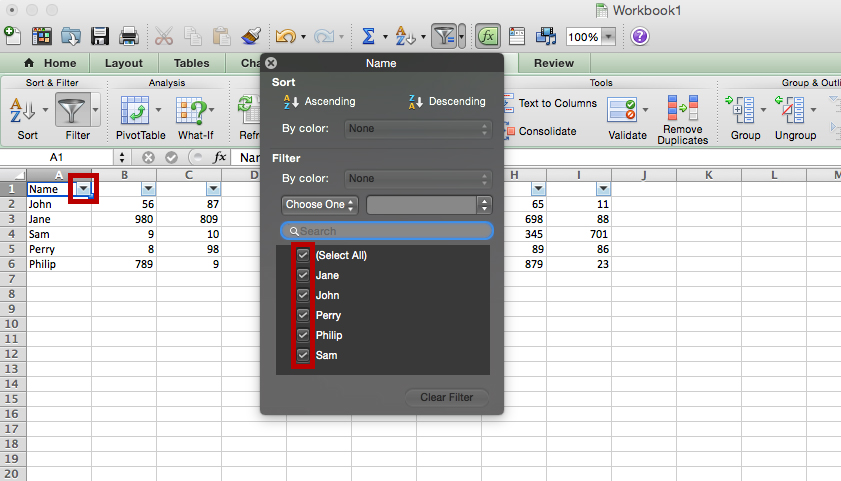
From the list that appears, you can choose certain values or names. Simply unclick “Select All,” and then click on the names you want. Once you hit “OK,” the dropdown menu will disappear and show you just the names you had selected.

The list has now been truncated to include the values you chose. But as you can see by the circled row numbers, the other data has not been deleted; it is simply “hidden” in this view.

You can easily undo any sorting by clicking on the Filter button at the top and choosing “(Select All)” again.

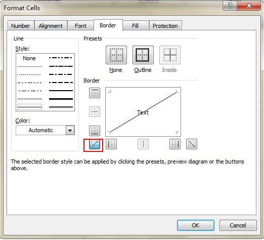
Add a Diagonal Line to a Cell

When creating a classmate address list, for example, you may need a diagonal link in the first cell to separate different attributes of rows and columns. How to make it? Everyone knows that Home->Font-> Borders can change different borders for a cell, and even add different colors. However, if you click More Borders, you will get more surprises, like a diagonal line. Click it and save—you can now make it immediately.

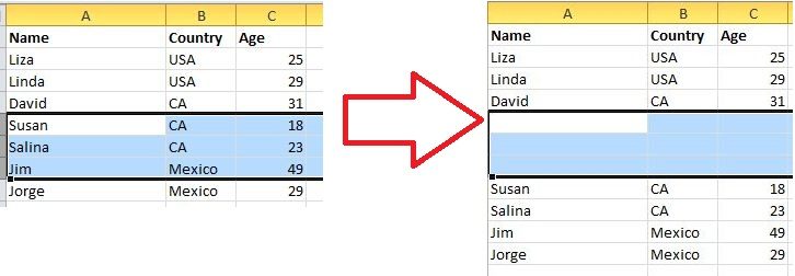
Add More Than One New Row or Column

You may know the way to add one new row or column, but it really wastes a lot of time if you need to insert more than one of these by repeating this action X number of times. The best way is to drag and select X rows or columns (X is two or more) if you want to add X rows or columns above or left. Right click the highlighted rows or columns and choose Insert from the drop down menu. New rows will be inserted above the row or to the left of the column you first selected. (ms excel tips)

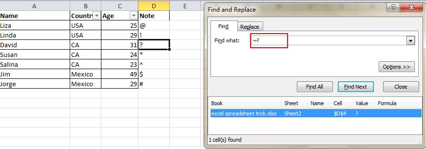
Vague Search with Wild Card

You may know how to activate the speedy search by using the shortcut Ctrl + F, but there are two main wild cards—Question Mark and Asterisk—used in Excel spreadsheets to activate a vague search. This is used when you are not sure about the target result. Question Mark stands for one character and Asterisk represents one or more characters. What if you need to search Question Mark and Asterisk as a target result? Don’t forget add a Wave Line in front.

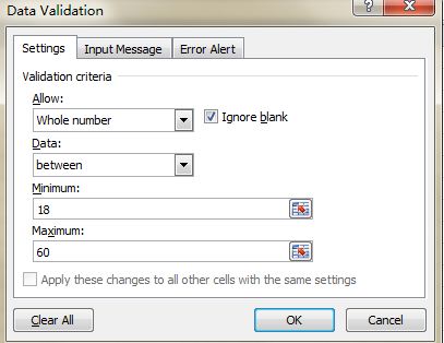
Input Restriction with Data Validation Function

In order to retain the validity of data, sometimes you need to restrict the input value and offer some tips for further steps. For example, age in this sheet should be whole numbers and all people participating in this survey should be between 18 and 60 years old. To ensure that data outside of this age range isn’t entered, go to Data->Data Validation->Setting, input the conditions and shift to Input Message to give prompts like, “Please input your age with whole number, which should range from 18 to 60.” Users will get this prompt when hanging the pointer in this area and get a warning message if the inputted information is unqualified.

Excel Formulas

Simple Calculations

In addition to doing pretty complex calculations, Excel can help you do simple arithmetic like adding, subtracting, multiplying, or dividing any of your data.

• To add, use the + sign.
• To subtract, use the – sign.
• To multiply, use the * sign.
• To divide, use the / sign.

You can also use parenthesis to ensure certain calculations are done first. In the example below (10+1010), the second and third 10 were multiplied together before adding the additional 10. However, if we made it (10+10)10, the first and second 10 would be added together first.

Simple Calculations

In addition to doing pretty complex calculations, Excel can help you do simple arithmetic like adding, subtracting, multiplying, or dividing any of your data.

• To add, use the + sign.
• To subtract, use the – sign.
• To multiply, use the * sign.
• To divide, use the / sign.

You can also use parenthesis to ensure certain calculations are done first. In the example below (10+1010), the second and third 10 were multiplied together before adding the additional 10. However, if we made it (10+10)10, the first and second 10 would be added together first.

Conditional Formatting Formula

Conditional formatting allows you to change a cell’s color based on the information within the cell. For example, if you want to flag certain numbers that are above average or in the top 10% of the data in your spreadsheet, you can do that. If you want to color code commonalities between different rows in Excel, you can do that. This will help you quickly see information the is important to you.

To get started, highlight the group of cells you want to use conditional formatting on. Then, choose “Conditional Formatting” from the Home menu and select your logic from the dropdown. (You can also create your own rule if you want something different.) A window will pop up that prompts you to provide more information about your formatting rule. Select “OK” when you’re done, and you should see your results automatically appear.